Difference-in-differences (DID) is a fantastic and widely-applied tool in the causal inference toolbelt. The idea is simple: you want to know if some sort of treatment, which was applied at time \(T\) to a “treatment group”, had an effect. You start by looking at whoever was treated and compare them after-\(T\) to before-\(T\), calculating the before-after “difference.”
However, we can’t just assume that the before-after difference is the effect of the treatment, since maybe things would have just changed over time anyway. We have a time effect clogging things up, and the before-after difference is a combination of the treatment effect and the time effect.
So we take a control group that didn’t get the policy and look at their before-after difference. We assume that their before-after difference is the before-after difference the treatment group would have gotten if the treatment had never occurred, i.e. this is our estimate of the time effect alone. We subtract out this control group before-after difference (the time effect) from the treatment group before-after difference (time effect + treatment effect), leaving us just with the treatment effect. And now we know the effect of treatment.
Parallel Trends
The key assumption holding this whole method together is parallel trends. We can describe parallel trends in all sorts of fancy ways, like “we assume that, if treatment had never occurred, the gap between treated and control groups would have remained constant from the before-treatment period to the after-treatment period.”
But really what parallel trends means is this: remember that “time effect” we talked about? Parallel trends says that the “time effect” for the treatment group is the same as the “time effect” for the control group. So when we subtract out the control group’s before-after difference, we’re subtracting the “time effect”, how much the treatment group would have changed over time anyway.
Now here’s the wild thing about parallel trends: it feels like you’re making some deep assumption about something structural and meaningful, something about the comparability of your treatment and control groups. But nope! It’s actually just a functional form assumption.
In fact, whether parallel trends is true or not is entirely based on which functional form you choose. This pops up most commonly in the decision of whether or not to take the log of your dependent variable in DID, since doing so could either fix or break your parallel trends assumption (or it could be broken either way).
For example, imagine that in the pre-treatment period, the treatment group has \(Y = 2\) and the control group has \(Y = 1\). In the post-treatment period, in the unobserved counterfactual where treatment didn’t occur, the treatment group has \(Y = 3\) and the control group has \(Y = 2\).
If the treatment hadn’t occurred, both groups would have increased by exactly 1 unit from before to after. Parallel trends holds! But what if we take the natural log of \(Y\)? Well, now, the treatment group increases by \(\ln(3)-\ln(2)\approx .405\) and the control group increases by \(\ln(2)-\ln(1)\approx .693\). Oops! Parallel trends is blown.
We Do What We Like
So parallel trends is a functional form assumption. So what?
So, that means it always holds. For the right functional form.
Like I said, it’s just a functional form assumption, not anything deep and structural about the data generating process. If we pick the right transformation, we can make parallel trends hold.
Thanking Ben Jackson for this particular specification, let’s pick the following transformation:
\[ F(Y, a) = (Y+a)^2 \]
Now, let’s specify our parallel trends assumption for a two-period DID. Let’s call \(Y_{gt}\) the outcome for group \(g\) ((T)reated or (C)ontrol) in time period \(t\) ((B)efore or (A)fter treatment).
\[ (F(Y_{TA},a) - F(Y_{TB},a) = F(Y_{CA},a) - F(Y_{CB},a)) \] which we can solve for \(a\)! We get:
\[ a = \frac{Y_{TB}^2+Y_{CA}^2 - Y_{TA}^2 - Y_{CB}^2}{2(Y_{TA}+Y_{CB}-Y_{TB}-Y_{CA})} \] So as long as \(Y_{TA}+Y_{CB}-Y_{TB}-Y_{CA} \neq 0\) (in other words, as long as the treated group didn’t rise from before to after by the exact same amount that the control group fell), we can always pick an \(a\) that gives us a transformation to make parallel trends true. Of course, actually picking the right \(a\) requires that we know the counterfactual \(Y_{TA}\), but we’ll get there later.
Let’s work a quick example. Let’s say that, in the before-treatment period, \(Y_{CB} = 1\) and \(Y_{TB} = 2\). Then, in the after-treatment period, \(Y_{CA} = 10\) and \(Y_{TA} = 8\). The control group rose by 9, and if treatment hadn’t occurred, the treated group would have risen by only 6. Parallel trends broken!
But using the formula above we can calculate \(a = -13/2\) and get our transformed values \(F(Y_{CB},a) = 121/4\), \(F(Y_{CA},a) = 49/4\), \(F(Y_{TB},a) = 81/4\), and \(F(Y_{TA},a) = 9/4\). Does parallel trends hold? We need
\[ \frac{9}{4} - \frac{81}{4} = \frac{49}{4} - \frac{121}{4} \]
for which you’ll find both sides are exactly \(-18\). Parallel trends holds.
I Will Punch It Until It Is True
So if we did know what the counterfactuals were, we could always pick an \(a\) that would make parallel trends true, if we used transformation \(F(x,a) = (x+a)^2\).
What if we don’t?
Well, dang, let’s just try a bunch of \(a\) values and see what we get! It sure would be interesting if we could just guess some \(a\) values from \(-5\) to \(5\) and get pretty close.
Let’s start by creating four random counterfactuals. For simplicity let’s keep them uniformly distributed in the range of 0 to 1. Then, let’s add a true treatment effect of .2. We’ll run things a bunch of times, picking a range of \(a\) values from -5 to 5 and see what we get. Wouldn’t it be wild if we tended to get accurate answers of .2 anyway?
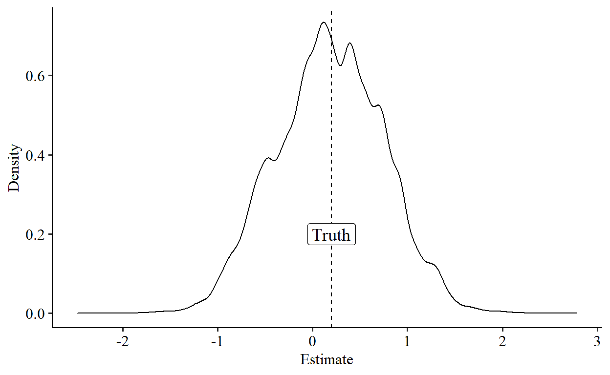
Um… what? To be entirely honest, I didn’t expect it to actually work. But look at that. I just picked a range of random \(a\) values to do the transformation on. And repeating the process I… I get a normal-looking distribution centered around the truth of \(.2\). Huh?
Okay, I’m cheating a little bit. The DID estimated using our transformation gives us an estimate on \(F(Y,a)\) scale, not on the \(Y\) scale where the truth is \(.2\). To get back to that scale I had to do a re-conversation, and it turns out that converting the DID estimate in \(F(Y,a)\) scale back to an estimate in \(Y\) scale leads you to a quadratic formula, so there are actually two solutions to what the DID estimate is in terms of \(Y\), and I picked the estimate closer to \(.2\). Cheating! Sorry. Let’s go ahead and undo that lil problem and look at both quadratic solutions:
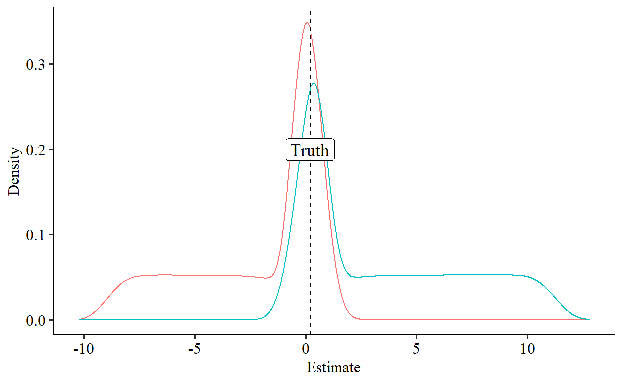
That still looks pretty good. Each of the solutions has one fat tail, but it’s still not bad. Um, this blog post wasn’t supposed to go this well. What happens if we average the two solutions for each run?
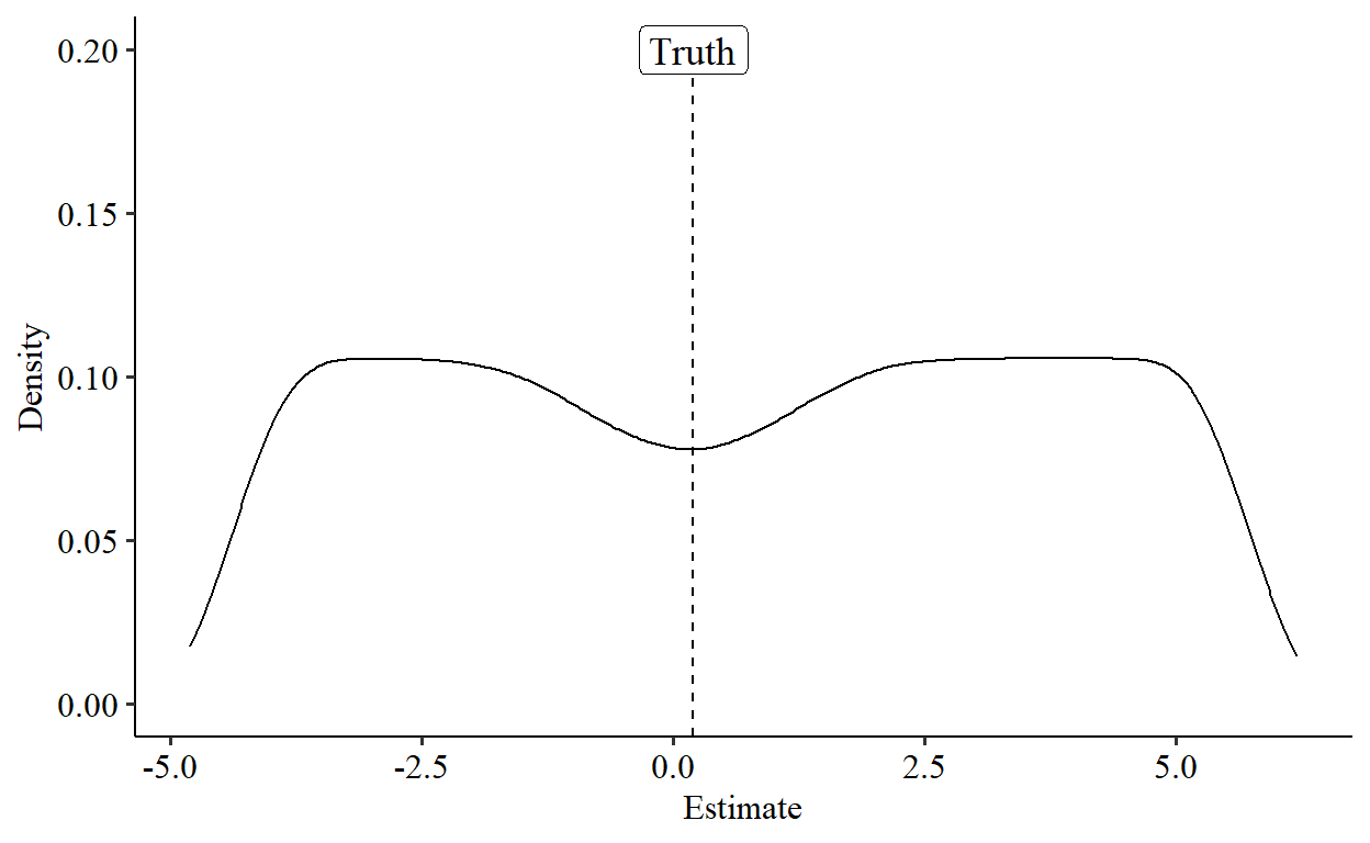
Now we get something that looks ugly, as it should be. Sure, the distribution is centered around the truth, but there’s no peak at the truth, in fact there’s a weird divot.
A Free Lunch?
But still, it sort of looks like if we knew which of the two quadratic solutions to pick, we’d have the ability to pick a functional form that made parallel trends true, and the ability to recover the original-value-scaled estimate, with a normal-looking sampling distribution centered around the true value.
Seems like in a lot of cases we could probably eliminate one of the two quadratic solutions by theory, say if one was positive and one negative (not guaranteed to happen). Hmm.
I’ll be honest, I’ve had a lot of ideas for causal-identification-by-magic in the past, and none of them have borne out. I expected this blog post to be the same. And yet! This is still looking pretty good so far. I’m sure there’s a reason bubbling just under the surface as to why this wouldn’t actually work (perhaps I’ve gotten lucky with the range of \(a\) values I picked) but for the moment I am keeping the magic alive and wondering what exactly about this must not work, so that I’m just fooling myself.
Or maybe not?