Ordinary least squares (OLS) is a statistical algorithm that uses a set of explanatory variables to predict a dependent variable. I dunno, maybe you’ve heard of it.
Describing what OLS does and what properties it has is often done in the form of mathematical statements. These statements are precise, and correct, and often confusing.
In this post I will translate several of these mathematical statements into the English language, giving a sense of what they actually mean in a non-technical sense. Sometimes I’ll add a graph if it helps.
Many of these translations can also be found on the more extended discussions of OLS in my book The Effect. So check that out. But I’ve decided to collect, or perhaps reiterate, some of them here. I’m not referring back to the book as I do this. If I have any here that I didn’t include in the book, oops.
As a note, this is all about translating precise mathematical statements into good ol’ imprecise English. Yes, these translations will miss some of the details. That’s in their nature. And if I included every caveat they would only become confusing. So no need to DM me about some caveat that the English translation leaves out. If you want full precision, just revert to the mathematical statements. If you just want a head start on understanding what OLS, uh, is, with the knowledge that some finger details may emerge later, forge on.
OLS Picks a Shape
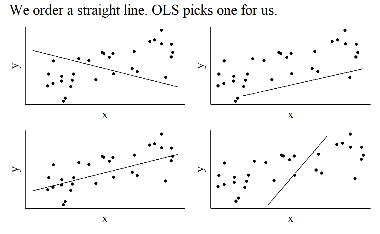
OLS is a tool that picks the best version of a shape. That’s all it does. That is, we tell it the kind of shape we want it to use, and we want it to tell us how to angle and move that shape to best fit the data.
What does that mean mathematically and in English? Mathematically, we might write down a regression equation that looks like this:
\[ Y = \beta_0 + \beta_1X+\varepsilon \]
In doing so, we are saying “OLS, give me the best straight line that describes my data,” since this equation describes a straight line with an intercept (\(\beta_0\)) and a slope (\(\beta_1\)). If we didn’t want a straight line - if we wanted a curvy line or something else, we’d need to rewrite this equation.
This also tells us how we can interpret our regression coefficients when we get them. They’re just describing a line, so we can interpret the coefficients as telling us how to move along that line.
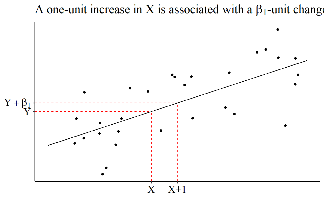
So the slope coefficient, \(\beta_1\), is just how steep the line is. Big positive numbers indicate a steep slope upwards, big negative numbers indicate a steep slope downwards, and numbers near zero indicate a flat line. More precisely, “a one-unit increase in \(X\) is associated with a \(\beta_1\)-unit increase in \(Y\).”
How OLS Picks a Shape
So we give OLS a shape and it picks the best version of that shape. How does it pick it? OLS picks coefficents that minimize the sum (\(\sum\)) of squared (\(^2\)) residuals (\(Y-\hat{Y}\)). With a single predictor \(X\) this means:
\[ \hat{\beta} = \text{argmin}_{\hat{\beta}}\sum_i(Y_i-\hat{Y}_i)^2 = \text{argmin}_{\hat{\beta}}\sum_i(Y_i - \hat{\beta}_0-\hat{\beta}_1X_i) \]
where \(i\) corresponds to the different observations. \(\hat{Y}_i\) is our prediction of the outcome variable \(Y\) for observation \(i\). If take \(X_i\) and look for where that \(X\) value falls on our OLS line (\(\hat{\beta}_0+\hat{\beta}_1X\)), that’s how we get our prediction \(\hat{Y}\). That prediction will, naturally, not be perfect, and so we’ll have a residual, which is the difference between the actual outcome \(Y\) and the prediction \(\hat{Y}\). We square those residuals (\((Y_i-\hat{Y}_i)^2\)), sum them up across all the observations (\(\sum_i\)), and then pick the line that makes that sum of squared residuals as small as possible (\(\text{argmin}_{\hat{\beta}}\)).
So what does this mean in English? It means that OLS is trying to pick the best line for you. Its idea of “best” is a line that makes predictions as close to accurate as possible. Since it can’t hit all the points perfectly, it has to trade off all the different errors in prediction for all its different predictions. It squares the errors in prediction, which both (a) makes sure too-high and too-low predictions are both bad, and (b) makes it try extra-hard to avoid predictions that are way off.
The Shape OLS Picks
If you solve the minimization problem in the previous section, you get the following estimate for the slope and intercept coefficients:
\[ \hat{\beta}_1 = \frac{Cov(X,Y)}{Var(X)} \] \[ \hat{\beta}_0 = \bar{Y} - \hat{\beta}_1\bar{X} \]
where \(Cov(X,Y)\) is the covariance between \(X\) and \(Y\), \(Var(X)\) is the variance of \(X\), and \(\bar{Y}\) and \(\bar{X}\) are the mean of \(Y\) and \(X\), respectively.
If we have more than one predictor, then with a matrix of predictors \(X\) and the associated coefficient vector \(\hat{\beta}\) we have
\[ \hat{\beta} = (X'X)^{-1}X'Y \]
Why does it make sense that these are the calculations we get? Let’s translate.
First, the slope of \(\hat{\beta}_1 = Cov(X,Y)/Var(X)\). There are a few ways we can think of this. It helps to first translate what “divides by” means. In statistical applications, \(A/B\) can usually be thought of as “how much \(A\) is there for each \(B\)?” or “out of all the \(B\)s, how many are \(A\)s?”
One way is “out of all the variation in \(X\) (\(/Var(X)\)), how much of that goes along with \(Y\) (\(Cov(X,Y)\))?” I think this translation is highly intuitive as a first step, although it becomes less so when you realize that \(\hat{\beta}_1\) can be outside of the range of 0 to 1 and so the implied-but-not-stated idea that this is a proportion isn’t accurate.1
Another way is “how much change in \(Y\) (\(Cov(X,Y)\)) can we expect relative to (\(/\)) how much \(X\) is changing (\(Var(X)\))? How much rise up the y-axis do we get as we run along the x-axis?
Whichever of these two translations you favor, their logic works just as well for the multivariable version \(\hat{\beta} = (X'X)^{-1}X'Y\). The inverse (\(^{-1}\)) just means “divide by”.
Oh, and don’t forget the intercept \(\hat{\beta}_0 = \bar{Y} - \hat{\beta}_1\bar{X}\). This one’s easy. It forces the average of \(Y\), \(\bar{Y}\), to be the same as the average prediction of the model. In other words, it says “hey OLS, whatever slope you think is best, I trust you. I’m just gonna go ahead and make sure that the predictions are right on average.”
OLS has an Error
A fully specified equation that you might use to set up a regression should always have an error term, which here is \(\varepsilon\):
\[ Y = \beta_0 + \beta_1X+\varepsilon \]
This error term is not the same as the residual. The residual is what we get if we actually get a sample of data, estimate our OLS coefficients, and compare the OLS predictions against the actual \(Y\) values. The error, on the other hand, is the difference between the actual \(Y\) value and what the OLS would predict if we had full population data.
An effective, if wordy, translation is this: “In truth, there’s a whole bunch of stuff that determines the value of \(Y\). The model we write out is telling us literally everything about what determines \(Y\) (that’s why it’s \(Y=\), not”\(Y\) is related to…“). Our model contains some stuff (\(X\)), but leaves out other stuff. That other stuff has to be somewhere, so it must be in the error (\(\varepsilon\)).”
OLS Can be Biased
If you want the estimated coefficient \(\hat{\beta}_1\) from \(Y = \beta_0 + \beta_1X+\varepsilon\) to reflect “the effect of \(X\) on \(Y\),” then we must assume that \(E(X\varepsilon) = 0\), where \(E()\) is the expectations function. \(E(X\varepsilon) = 0\) means that there’s no linear relationship between \(X\) and \(\varepsilon\).
If that’s not true, and \(E(X\varepsilon) \neq 0\), then we have omitted variable bias. Some variable that’s related to \(X\) has been omitted from the model and thus is in \(\varepsilon\) (remember last section? Every determinant of \(Y\) that’s not in the model is in \(\varepsilon\)).
If we estimate a regression based on the model \(Y = \beta_0 + \beta_1X+\varepsilon\), but there’s a variable \(Z\) in the error term \(\varepsilon\), the estimate we get will be
\[ \hat{\beta}_1 = \beta_1 + \beta_Z\beta_{XZ} \]
where \(\beta_Z\) is the coefficient we’d get on \(Z\) if we instead estimated a regression of \(Y\) on both \(X\) and \(Z\), and \(\beta_{XZ}\) is the coefficient we’d get on \(Z\) if we regressed \(X\) on \(Z\).
How can we translate this?
“If \(Z\) tends to hang around \(X\) (\(\beta_{XZ} > 0\)), but OLS doesn’t know about it (\(Z\) isn’t in the model), then \(X\) will get the credit for everything \(Z\) actually did (\(\beta_Z\)).”
The same idea holds if \(X\) and \(Z\) are negatively related (\(\beta_{XZ} < 0\)), although it’s not quite as intuitive:
“If \(Z\) tends to disappear when \(X\) is around (\(\beta_{XZ} < 0\)), but OLS doesn’t know about it (\(Z\) isn’t in the model), then \(X\) will get blamed for \(Z\) not doing what it normally does (\(\beta_Z\)).”
The Precision of OLS
Since we often want to use our OLS estimates to make inferences about the population, we want to have an idea of what the sampling distribution of OLS is.
In the regression following from the model \(Y = \beta_0+\beta_1X+\varepsilon\), if we assume that \(\varepsilon\) has a constant variance \(\sigma^2\), then the sampling distribution of our estimate \(\hat{\beta}_1\) is centered around the population value of that coefficient \(\beta_1\), and has a standard deviation of
\[ se(\hat{\beta}_1) = \sqrt{\frac{\sigma^2}{Var(X)}} \]
or in the multivariable context, the very similar
\[ Var(\hat{\beta}) = \sigma^2(X'X)^{-1} \]
where \(se(\hat{\beta}_1)\) is then the square root of the first element of the trace of \(Var(\hat{\beta})\).
How can we interpret this? Well, we have a standard error that grows the more the error term varies (\(\sigma^2\)), and shrinks the more \(X\) varies (\(/Var(X)\)). The error term contains all the other stuff going on with \(Y\) other than what’s in the model. So we can say “The difficulty in figuring out exactly what our slope coefficient is is based on how much other stuff there is going on with \(Y\) (\(\sigma^2\)) relative to the parts we’re actually interested in (\(Var(X)\)). The more noise there is relative to signal, the less we can see, and the less precise we’ll be.”
There’s another few steps (and another translation) to go here for when we want to get a little dirty. First, keep in mind that whatever the standard error is, we don’t actually know it, we have to estimate it just like we have to estimate the coefficient itself. We can make an estimate of \(\hat{\sigma}^2\) using the variance of the residuals. Second I gave the equations for standard errors if the error term has a constant variance. However, if we don’t make that assumption, then instead of the nice simple \(\sigma^2\) we have \(E(\varepsilon\varepsilon')\), which is the variance-covariance matrix of the error terms.2 Estimating the standard error, then, means we have to try to estimate \(E(\varepsilon\varepsilon')\) in its entirety,3 Things like heteroskedasticity-robust or cluster-robust standard error estimations make different assumptions about \(E(\varepsilon\varepsilon')\) in order to more precisely estimate it.
What does this mean?
“How precise our estimate is depends on how much noise there is. If we’re wrong about how much noise there is, we’ll also be wrong about how precise our estimate is. If the noise isn’t just a single thing but instead changes a lot, we have to do something to figure out how it changes, or we’ll be wrong.”
Although this same interpretation works much better for Pearson correlation, which is basically a univariate regression coefficient rescaled so it’s much more proportion-like.↩︎
The entire equation itself gets a bit gnarlier too, since \(\sigma^2\) lets some stuff cancel out and we don’t get that any more. In the multivariable context it’s \((X'X)^{-1}(X'E(\varepsilon\varepsilon')X)(X'X)^{-1}\).↩︎
Or at least that’s what sandwich-based estimators do.↩︎