Identification via Heteroskedasticity
Note: after posting this on Twitter it became very apparent that I did not invent this idea, and if you want to explore it further I recommend a number of papers by Arthur Lewbel on this topic. But perhaps you will still find the intuitive explanation here useful.
In this article I will produce a sketch to demonstrate an entirely new approach to identifying a causal effect that relies on an entirely different set of assumptions from what you’d normally see. Why am I introducing this via blog rather than in an academic publication? Simply, if I put the time into developing this into an academic publication, I can tell you exactly what the reviewers would say: “okay, sure, but in what context do these different assumptions actually hold?” and I’d give a big ol’ shrug because I don’t know. I still think it’s pretty neat if only as a curiosity. And hey, if you’re out there and thinking “hold on, I do actually know a context where this can be applied!” then please do get in contact with me. I’d love to hear about it, and maybe then I’d turn this into a paper.
At this point, it’s really just an idea.
The basic idea begins with the basic way we usually identify the causal effect of \(X\) on \(Y\), which is through the use of assumptions about variables being unrelated. You almost always need one (or more) of these assumptions to be able to identify a causal effect. If you want to simply estimate the relationship between \(X\) and \(Y\) and say “this relationship describes the causal effect of \(X\) on \(Y\)” you need to make an assumption similar to “the other determinants of \(Y\) that are not themselves determined by \(X\) are all unrelated to \(X\)”.
This assumption is actually stronger than we need it to be. What we actually need, in a regression for example, is that variables are uncorrelated. This is not as strong a requirement as being unrelated, since “uncorrelated” only cares about linear dependence. If the graph with \(Y\) on the y-axis and \(X\) on the x-axis has the shape of a U, for example, then \(X\) and \(Y\) are clearly related, but are uncorrelated.
We’re used to assumptions about things being uncorrelated. When thinking through a causal analysis that uses regression, we constantly ask whether the mean of the treatment variable \(X\) is likely to be higher or lower based on the value of some variable that’s been excluded from the regression.
We think about other elements of two variables being related besides correlation in some ways too. We think about heteroskedasticity, which is the relationship between \(X\) and the variance of the error term (which consists of terms excluded from the regression). Heteroskedasticity isn’t important for identifying the effect, but we do need to keep it in mind when calculating standard errors.
But what if we could flip that? What if assumptions about heteroskedasticity were what we used to identify our effect, and assumptions about correlation weren’t important?
This is possible under the right assumptions!
The Basic Idea
The insight here is that heteroskedasticity allows you to pick up a causal effect (or at least its magnitude) in a sort of dose-response kind of way. Intuitively, if you make the treatment more noisy, then if there’s a causal effect, the outcome should get more noisy at the same time. We can detect the extent to which this happens by comparing variances. That’s it, that’s the idea.
A Mathematical Demonstration
Let’s do a demonstration. We are trying to get the effect of \(X\) on \(Y\), both continuous and mean-zero. However, there are two confounders, one binary observed confounder \(Z\) and one unobserved confounder \(W\). The data generating process is as follows:
\[ X = \gamma_z Z + \gamma_wW + \nu \]
\[ Y = \beta_x X + \beta_z Z + \gamma_wW + \varepsilon \]
\[ \nu \sim N(0, \sigma^2_X \equiv 1 + Z\theta_{xz} + W\theta_{xw}), \varepsilon \sim N(0, \sigma^2_\varepsilon) \]
If we use a method that relies on \(E(XW)=E(X)E(W)\), like regressing \(Y\) on \(X\) and \(Z\) and looking at the coefficient on \(X\), we’ll be biased, since \(X\) and \(W\) are correlated.
But what if, instead, we look separately at the \(Z = 0\) and \(Z = 1\) groups. Then, in those groups, we examine the variance of \(Y\). We’ll start with the variance of \(Y\), assuming that \(\varepsilon\) is independent of everything.
\[ Var(Y) = \beta_W^2\sigma^2_W + \beta^2_Z\sigma^2_Z + \beta^2_X\sigma^2_X + 2\beta_W\beta_Z\sigma_{WZ}+2\beta_W\beta_X\sigma_{WX}+2\beta_Z\beta_X\sigma_{ZX}+\sigma^2\varepsilon \]
We’ll take this separately conditional on \(Z = 1\) and \(Z = 0\) and differencing (under the assumption that treatment effects do not vary between \(Z = 1\) and \(Z = 0\)):
\[\begin{eqnarray} Var(Y|Z=1) - Var(Y|Z=0) = \beta^2_W(\sigma^2_{W|Z=1}-\sigma^2_{W|Z=0}) + \beta^2_X(\sigma^2_{X|Z=1} - \sigma^2_{X|Z=0}) + \\ 2\beta_W\beta_X(\sigma_{WX|Z=1}-\sigma_{WX|Z=0}) \end{eqnarray}\]
Let’s replace all those differences in variance and covariance between \(Z = 1\) and \(Z = 0\) with \(d\) for notational simplicity, i.e. \(dA = Var(A|Z=1)-Var(A|Z=0)\) and \(dAB=Cov(A,B|Z=1)-Cov(A,B|Z=0)\). Then rearrange.
\[ 0 = \beta_X^2dX + 2\beta_W\beta_XdWX + (\beta^2_WdW - dY) \]
This is a quadratic in \(\beta_X\) and so we can solve it with the quadratic formula.
\[ \beta_X = \frac{(-b\pm \sqrt{b^2-4ac})}{2a} \]
\[ \beta_X = \frac{(-2\beta_WdWX\pm \sqrt{(2\beta_WdWX)^2-4dX(\beta^2_WWdW - dY)})}{2dX} \]
All the terms with \(W\) are unobservable, but the rest are observable. Let’s assume that \(dWX=dW=0\). That is, \(W\) and \(X\) may be correlated, but that degree of correlation is not related to \(Z\). Further, the variance of \(W\) is not related to \(Z\) (although potentially \(Z\) and \(W\) may be related, that’s fine). This gives us
\[ \beta_X = \frac{\sqrt{dY}}{\sqrt{dX}} \]
\[ \beta_X^2 = \frac{dY}{dX} \]
That’s riiiight, it’s a Wald estimator! Derived from the quadratic formula! In this setup, you’re basically using \(Z\) as an instrument for \(\sigma_X^2\). That’s where the necessary assumptions come from, they’re just all about variances rather than means. It’s ok if \(Z\) is related to \(W\) just so long as \(Z\) is unrelated to \(\sigma_W\) (the \(dW=0\) assumption).
Now we have the magnitude of \(\beta_X\) - it’s \(\frac{\sqrt{dY}}{\sqrt{dX}}\). We don’t get the sign, but we generally have a pretty strong theoretical idea of what a sign should be, and the magnitude (or whether that magnitude is nonzero) is more the question.
Notably, also, this could all be done with a discretized continuous Z, i.e. “pick two groups for which \(\sigma_X\) is different, using \(Z\) to identify those groups”.
Simulation
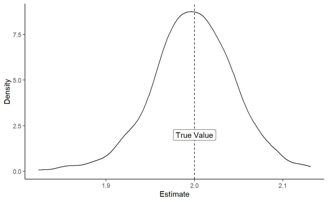
I haven’t worked out a more nonparametric or nonlinear version of this, but that’s the basic idea. It works in simulation, too (and yes, 2SLS is an equivalent way to derive this in the linear case, and you get SEs).
In the sampling distribution you can see that the mean and median are both bang-on to the true value of 2. The standard deviation of the sampling distribution ain’t shabby either.
| Variable | N | Mean | Std. Dev. | Min | Pctl. 25 | Pctl. 50 | Pctl. 75 | Max |
|---|---|---|---|---|---|---|---|---|
| rat | 500 | 1.998 | 0.047 | 1.824 | 1.97 | 1.998 | 2.03 | 2.131 |
Conclusion
What can we get from all of this?
Well, I think it’s kind of neat that this offers a potential way to identify a causal effect without so many of the assumptions that we typically rely on and seem impossible to get around without some sort of quasiexperimental design.
At least the way I’m thinking about it, this is basically a way of managing to control for unobserved confounders using observed confounders.
Of course, that’s not entirely true. You could call this a quasiexperimental design, really. I mean, it reduces mathematically to 2SLS at least in some formulations. But the assumptions that stand in here for the exclusion restriction feel so different that it seems like a very different kind of thing.
There are the downsides, of course. The obvious one being “where the heck would we expect these assumptions to hold?” The variance of treatment is related to the value of another, sure. But we aren’t used to thinking about no-heteroskedasticity assumptions, i.e. the assumption here that the variance of the unobserved confounder \(W\) is unrelated to \(Z\) (and in a case where maybe even the mean of \(W\) is related to \(Z\)! Since if that’s not true we may as well just use regular IV).
I’m not even sure the downside here is how unlikely the assumptions are so much as I’m not even sure how to reason about where I’d expect these assumptions to hold. I have too much experience working with uncorrelatedness assumptions. I’m not sure what a “the unobserved confounder’s variance is unrelated to this other variable’s value” assumption feels like or how to judge whether that assumption is plausible.
So maybe it’s just sorta neat rather than useful. This process feels a little like cheating, and I love a statistical method that feels like cheating. Plus I got to derive a Wald from the quadratic, which was fun. Then again, the different kind of assumption it calls for suggests that maybe there are situations where this applies, and I just don’t know where to look for them yet! Let me know if you think of one!